Do We Still Have to Denormalize? Have Your Schema and Search It Too


Search usually means returning results sorted by relevance (like BM25 or vector similarity), or summarizing results into facets. ParadeDB already makes this fast when your data lives in a single denormalized table.
But in a relational database, data is usually normalized and factored out into separate tables, like users, posts, and comments. We call searching across multiple joined tables a search join, and making these queries fast is harder than it looks!
Historically this pattern left people either choosing speed, and denormalizing via a fragile ETL process into Elasticsearch1, or choosing simplicity and accepting Postgres2 slowly scoring and joining millions of rows only to return a handful of results.
We've spent the last few months making search joins a first-class experience in ParadeDB, removing the need to choose between complexity and slow queries. In our StackOverflow benchmark, a multi-table search query is up to 1000x faster than vanilla Postgres (dropping a natural 3-table Top-K search from 2 minutes to 100 ms), without the burden of any additional infrastructure.
Why Search Pushes You to Denormalize
To see what a search join looks like in practice, consider StackOverflow's data model, which exercises both relational joins and search: users (2.3M rows), posts (20M rows), comments (29M rows), and badges (29.4M rows), all of which should be easily accessible from a search box or agent.
Your instincts tell you that when you store this dataset in a database, most of it should be normalized: you don't want to denormalize users into their posts and comments and then need to update every post or comment they've ever made when they update their profile. When someone searches, you just want to write a single query that finds matches across users, posts, and comments, ordered by their combined relevance scores:
SELECT
  users.id AS user_id,
  users.display_name,
  posts.id AS post_id,
  posts.title,
  comments.id AS comment_id
FROM
  users
  JOIN posts ON users.id = posts.owner_user_id
  JOIN comments ON comments.post_id = posts.id
WHERE
  users.about_me ||| 'ocaml'
  OR posts.title ||| 'ocaml'
  OR comments.text ||| 'ocaml'
ORDER BY
  pdb.score(users.id)
    + pdb.score(posts.id)
    + pdb.score(comments.id) DESC,
  comments.id DESC
LIMIT 20;
But a traditional search engine tells you you can't write it this way. If you try to export to Elastic, then you'll wade through "nested field types", "enrich processors", "terms lookup queries", "runtime fields", "LOOKUP JOIN" with its 10,000-row batch circuit breaker, "client side _update_by_query", and "join fields" (only one per index!) before realizing that you still have to choose to denormalize either users or badges into every post and comment. And when you do denormalize, power-law skew makes the write and space amplification much worse than average row sizes suggest.3 Not only are you double writing into two databases, but the denormalized copy takes up to 3x the storage after replication.
Why Search Joins Are Slow in Postgres
What if you skip the external search engine and run that query directly in vanilla Postgres? On a B-Tree + GIN schema (with 8-way parallelism), it takes ~2 minutes (118,000 ms).
"Just Use Postgres" is a temptingly simple answer: but making it possible with minimal compromise requires rethinking how Postgres both indexes and executes queries. We've previously discussed how ParadeDB's indexes maintain transactional consistency, and how they outperform built-in indexes for single-table Top-K: but joins sit above individual indexes, inside Postgres's query executor.
Executing a search join quickly requires accessing the smallest amount of data you can (in a locality friendly manner) before a Top-K or aggregate above the join reduces its volume to something that can comfortably be rendered for your users. In this case the bounded output (a small LIMIT or GROUP BY) is a critical portion of the problem.
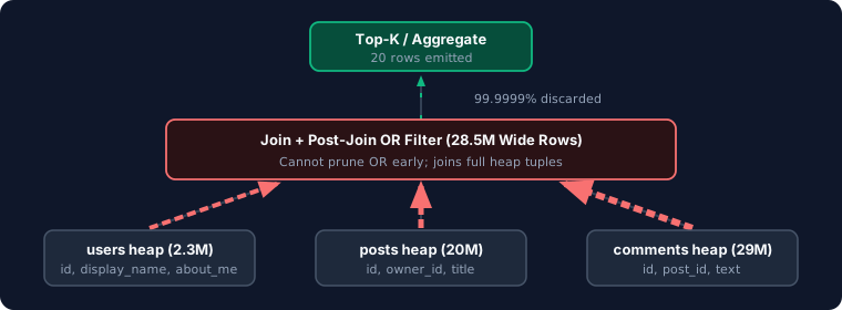
When you sort by a single column like created_at, Postgres could walk a B-Tree index and finish once it has found 20 qualifying rows. When you sort by the sum of relevance scores across OR'd tables, no tables are pre-ordered by that combined score. Because a comment without 'ocaml' might still match via its post or user, Postgres can't even filter the tables before joining them. It has to join all 28.5M rows first, sum the scores for every triple, and only then sort and take the top 20.
Processing all these rows is expensive, because Postgres's row-at-a-time executor needs to fetch a tuple from the table storage (the heap) to join on. When it fetches that tuple, the cost of doing so is high enough that Postgres will always fetch all columns that might be needed for the query (display_name, title, etc.): even if the row is very likely to be eliminated later by the LIMIT 20.
For aggregate queries, Postgres's lack of vectorization and the need to pick single columns out of the heap similarly hamper its performance. Covering B-Tree indexes (usually specialized for the particular aggregate you need to execute) can help, but degrade write throughput as they accumulate (by introducing random writes in your insert path), and can't approach the aggregate performance of a column store.
Specialized query rewrites (such as rewriting the OR as an 84-line UNION ALL of separate per-table queries in a CTE) can get you closer: down from ~2 minutes to 1.2s for a rare search term, but they're much more code to maintain, and for a common term the runtime balloons to 14s.
Getting that original, natural SQL query down to 100 ms on a single core (12x-50x faster than the 84-line UNION ALL rewrite, and within range of a fully denormalized dataset) required rethinking how joins and search indexes interact.
Building an Executor for Search Joins
ParadeDB's index unifies columnar storage with BM25 and vector search, storing join keys and projected columns directly inside the index across the queried tables.
To execute joins directly over that columnar data (rather than tuple-at-a-time against the Postgres heap), using Postgres's executor was not an option. Instead, after recognizing a search join we intercept the query plan via Postgres's query planner hooks and propose a query path that pushes the entire multi-table JOIN and LIMIT / GROUP BY (and DISTINCT, OVER, FILTER etc) query to our columnar executor, built with Apache DataFusion. All of your non-search queries continue to use Postgres's standard planner and executor untouched, and for the queries we do accelerate, we extensively property test to ensure equivalence to Postgres.
DataFusion is one of the fastest OLAP query engines available today: it's built around vectorized execution, and its shared-nothing model is a perfect fit for Postgres's process model.4
But one of DataFusion's most critical features for ParadeDB is its extensibility. To turn an analytical engine into a low-latency, transactional executor inside Postgres, we extended DataFusion so that only compact internal document IDs and join keys flow through joins (deferring column fetches until the right moment via selective late materialization56), and so that Postgres MVCC visibility checks are deferred until after joins have narrowed the rows (checking Postgres's in-memory Visibility Map before ever touching the heap).
Today, this executor is significantly faster than vanilla Postgres across the join shapes you encounter in a search workload.7 Below, we'll look at benchmarks and under-the-hood mechanics for the two query shapes that power almost every search page:
- Joining and sorting by relevance (Top-K): finding the top 20 results ranked by combined score across
OR'd tables, powered by a new operator introduced in 0.26.4 called a Rank Join. - Joining and grouping into facets (Aggregates): counting matching categories across
OR'd tables without touching the heap, powered by tuple tagging, index co-partitioning, and late materialization.
Joining and Sorting by Relevance (Top-K)
As we saw earlier, our original 3-table OR query forces vanilla Postgres to either join all 28.5M rows before filtering (~118,000 ms), or maintain an 84-line UNION ALL rewrite (1.2s to 14s, which effectively executes the join three times on common terms).8
ParadeDB 0.26.4 uses a Rank Join to execute the original, natural SQL in 100-600 ms on a single core across all selectivity levels:
Three-table Top-K search
Runtime · Log scale · Lower is faster
Each tick is 10× the previous tick.
| Query plan | ocaml (rare)0.06% / 17K matches | python (medium)5.3% / 1.5M matches | code (common)16.6% / 4.7M matches |
|---|---|---|---|
| ParadeDB 0.26.4 (Rank Join) | 101 ms | 603 ms | 274 ms |
| Postgres 84-line UNION ALL | 1,242 ms | 3,564 ms | 14,044 ms |
| Postgres natural SQL | ~118,000 ms | 118,010 ms | ~118,000 ms |
Postgres plans above execute in parallel across up to 8 workers; ParadeDB's Rank Join currently runs on a single core (see the benchmark harness).
How It Works: Rank Joins
How do you find the top 20 combined scores across joined tables without joining all 28.5 million rows first? Instead of joining the tables completely and sorting at the end, a Rank Join streams its inputs in descending score order (sorted access, or SA), building candidate result-sets as it goes. The lowest score seen in each stream is its SA floor, if the users stream reaches a SA of 4.0, no unseen user can score above 4.0. A post scoring 6.0 before author ss scored can therefore have a combined score of at most 10.0. This lets the executor stop early once it can prove that no remaining combination can beat its current top 20 results.
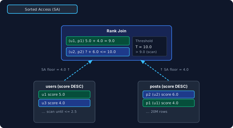
Consider joining just users and posts on users.id = posts.owner_user_id. In their most basic form9, Rank Joins use Sorted Access (SA) to pull top-scoring users and posts from each table's sorted score iterator into a hash table and candidate heap (u1: 5.0 and u3: 4.0 from users; p2: 6.0 and p1: 4.0 from posts).
When both sides of a pair have been seen, like (u1, p1), the heap knows its exact combined score (5.0 + 4.0 = 9.0).
When only one side has been seen so far, like post p2 by author u2 ((u2, p2)), the heap tracks it as a partial candidate, using the lowest score seen so far in the users stream (4.0) as an upper bound on u2's score (? + 6.0 ≤ 10.0).
Once enough rows have been pulled that no partial or unseen pair's upper bound (threshold) can beat the best complete pair in the heap (Threshold Met), it is safe to emit (u1, p1) as the next highest-scoring joined tuple.
The problem with this basic form is that when scores decrease slowly, or a high-scoring post like p2 (score 6.0) was authored by a user u2 who didn't match the search term at all (score 0.0, and so will never appear in the users SA stream), thousands of rows must be pulled in SA order just to push the users stream floor down low enough (≤ 2.5) to prove (u2, p2) cannot beat 9.0.
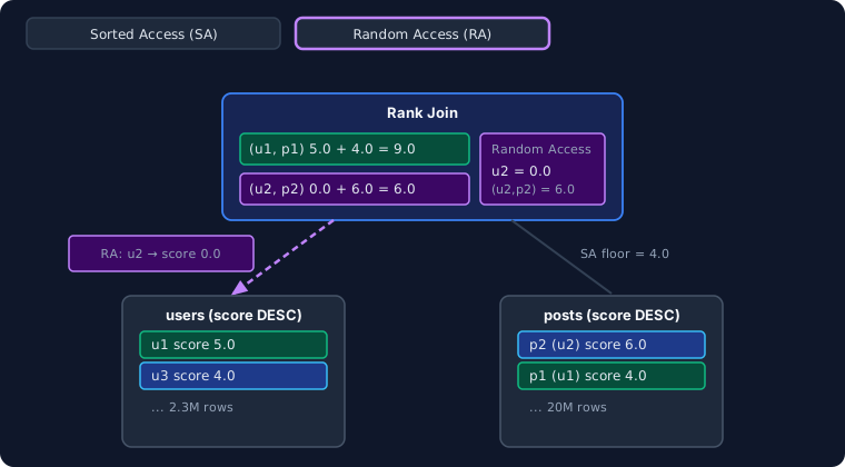
To fix this, further research10 added random access (RA) between the SA pulls and the threshold check: the best partial candidates in the heap trigger direct point lookups into the opposite table's index by join key (users.id = u2) to fetch their partner's exact score (0.0 if non-matching).
Resolving (u2, p2) early using RA (0.0 + 6.0 = 6.0) eliminates the only potential score above 9.0, satisfying Threshold Met (4.0 + 4.0 = 8.0 < 9.0) and emitting (u1, p1) while the SA streams are still at the very top.11
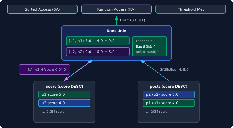
We implemented a streaming binary join operator in DataFusion, which means downstream operators can pull joined tuples until the stream ends: whether they exit early on a LIMIT 20 stopping after 20 rows, or drive a second stacked Rank Join ((users JOIN posts) JOIN comments) consuming as much as it needs to satisfy the three-table hierarchy. In future versions, we will support parallelizing and co-partitioning this operator across workers for even lower runtimes.
In ParadeDB 0.26.4, the result is a fully transparent binary join operator that allows for 100 ms three table OR Top-K queries (with projected columns like users.display_name and posts.title only materialized for the final 20 rows)... all with the most obvious and maintainable query that you can write.
Joining and Grouping Into Facets (Aggregates)
The other half of a search page is aggregates (often called "facets"), which summarize the full set of matches into category counts: like the brand, color, or size breakdown in an e-commerce sidebar.
Like a Top-K query, a facet query returns a small result ready to be rendered above the fold. Unlike Top-K, an aggregate has to count every matching row rather than stopping after the top 20: which means Rank Joins aren't the answer here.
In our StackOverflow search experience, right next to the Top-20 search results we want to render a sidebar of the top 10 tags across matching posts: where a post matches if 'python' appears in either the author's about_me or the post's title (854K matching posts across 20M total posts and 2.3M users):
SELECT
  posts.tags,
  COUNT(*) AS post_count
FROM
  users
  JOIN posts ON posts.owner_user_id = users.id
WHERE
  users.about_me ||| 'python'
  OR posts.title ||| 'python'
GROUP BY
  posts.tags
ORDER BY
  post_count DESC
LIMIT 10;
Because an aggregate must count all 854K matches rather than stopping after 20 rows, both Postgres and ParadeDB execute a parallel hash join across the 20M posts and 2.3M users before applying the OR filter. In Postgres a standard SQL JOIN takes 35.3 seconds scanning the heap, while a manual UNION rewrite (which must deduplicate posts.id to avoid double-counting posts) gets down to 1.0s across 2.33M buffers.
In ParadeDB, the natural SQL query runs entirely inside the columnar index in 422 ms, hitting 48x fewer buffers:12
Joining and counting facets
python · 854K matching posts
Log scales · Lower is better
Each tick is 10× the previous tick.
| Query plan | Runtime | Total buffers |
|---|---|---|
| ParadeDB natural SQL | 422 ms | 48.9K |
| Postgres UNION rewrite | 999 ms | 2.33M |
| Postgres natural SQL | 35,270 ms | 2.32M |
All plans above execute in parallel across up to 8 workers (see the benchmark harness).
How It Works: Tuple Tagging, Co-Partitioning, and Late Materialization
Three techniques in our executor combine to make this hash join and aggregate fast without touching the heap:
- Tuple tagging13 handles the
ORfilter: during the index scan on each table, each row is tagged with a 1-bit flag indicating whether it matched 'python', so the post-join filter (tag_users OR tag_posts) is a simple in-memory bitmap check. - Index co-partitioning via
partition_byaccelerates the hash join itself: when both indexes are partitioned by the join key (note: partitioning indexes, not tables: more on this in a future post!), each parallel worker is assigned a balanced range of join keys to join locally with zero contention (dropping runtime from 935 ms to 422 ms). - Selective late materialization accelerates the
GROUP BYabove the join: ParadeDB defers fetchingposts.tagsuntil aftertag_users OR tag_postshas pruned 20M posts down to 854K matches, aggregates locally on compact 8-byte dictionary ordinals, and only decodes the winning tag strings. And because ParadeDB's index is LSM-tree-based, adding extra facet columns to the index (>32 columns? go for it!) does not add random write traffic.
Have Your Schema and Search It Too
We set out to improve search joins because almost every user interested in ParadeDB asks about them first: "Can I have my normalized schema and search it too?". We believe that we've significantly shifted how often you can say "yes" to that question, helping our users to "Just Use Postgres".
A normalized data model might be the right choice for your application. But if you decide that you need to denormalize, ParadeDB is also one of the fastest single table search solutions, and a general-purpose, transactionally consistent database that also knows how to search is the best place to duplicate things!
We'll continue to push the performance of low-latency search and analytical queries over normalized data forward. If you'd like to test these queries on your own data, try ParadeDB Cloud or run ParadeDB locally, and stay tuned for more!
Footnotes
-
Search engines like Elasticsearch are fast, but require painful denormalization hoops. They have historically avoided joins and query optimization because their immutable, LSM-tree like architectures can absorb the huge batch writes required to update denormalized data as sequential segment writes, while providing low latency reads. ↩
-
Relational databases like Postgres support normalized schemas and joins natively, but struggle when relevance scoring is involved in the join. Postgres historically encouraged normalization to help more of your dataset fit in RAM and to reduce transaction sizes atop B-Trees (which dislike random writes), but its indexes and executor have no way to find the top results of a multi-table search without joining and scoring everything first. ↩
-
Prolific StackOverflow authors have 5x longer
about_mebios and 16x more badges per post than average. ↩ -
Multi-worker execution across Postgres background workers is powered by the datafusion-distributed contrib project. ↩
-
Liu et al. 2024 ("Selective Late Materialization in Modern Analytical Databases"). ↩
-
In
AND'd joins, dynamic join filters are also pushed from the build side into the probe side's index scan to prune rows before they ever leave the index. ↩ -
Even on Top-K joins ordered by a static column rather than relevance score (where Postgres can use a B-Tree index with a nested loop join), using a Rank Join like an index-backed nested loop join brings ParadeDB within an order of magnitude of native B-Tree nested loops, without the random writes of per-column indexes. ↩
-
If you let a frontier LLM loose to hyperoptimize a single SQL query for one specific search term atop B-Tree and GIN indexes, it will produce a 134-line, hierarchy-coupled, 7-match-state
LATERALwonder: and it will be faster for that exact query (34 ms), before ballooning to 16.6s at other selectivity levels. Because no one would maintain that in production, we've excluded it from the chart. ↩ -
Fagin, Lotem, & Naor 2001 ("Optimal Aggregation Algorithms for Middleware"). ↩
-
Bruno, Gravano, & Marian 2002 ("Evaluating Top-k Queries over Web-Accessible Databases"); Chang & Hwang 2002 ("Minimal Probing: Supporting Expensive Predicates for Top-k Queries"); Ilyas, Aref, & Elmagarmid 2004 ("Supporting Top-k Join Queries in Relational Databases"). ↩
-
This also explains the counterintuitive result in the chart above, where the common term 'code' (4.7M total matches, 274 ms) executes more than 2x faster than 'python' (1.5M matches, 603 ms). Because 'code' is so frequent, triples that match in all three tables appear densely near the top of each SA stream, driving the Top-K heap threshold up quickly: 'code' converges after scoring only ~9K total rows across the three tables, whereas 'python' has to score ~18K rows before proving no unseen combination can beat the top 20. ↩
-
Even on
ANDor single-table filtered joins where Postgres can use an index before the join (such as counting the top 10badgesacross 170.9K 'python' posts, which fan out 80x into 13.7M badge rows), ParadeDB executes the facet aggregate in 299 ms vs 2,225 ms in Postgres (664 ms if you create a dedicated coveringbadges(user_id, name)B-Tree, which still hits 122x more buffers than ParadeDB). ↩ -
Kim & Maden 2024; Candea, Polyzotis, & Vingralek 2009 ("A Scalable, Predictable Join Operator for Highly Concurrent Data Warehouses"). ↩