Teaching Postgres to Facet Like Elasticsearch

Picture this: you've built a perfectly reasonable search app. Users type "dinosaur," get results, everybody's happy. Then someone asks, "but how many of these are carnivores?" So you add filters. Then they want to know how many results each filter would give them before they click it. Welcome to Jurassic park faceted search.
In this post, we'll break down how we brought Elasticsearch-style faceting directly into PostgreSQL; the syntax, the planner integration, and the execution strategy that makes it possible. We'll show you how we structured the SQL API using window functions, and the results we can get from pushing as much work as possible down into our underlying search library (spoiler alert: over an order of magnitude faster for large result sets).
If you aren't familiar with ParadeDB, we're a Postgres extension that brings modern search capabilities directly into your database. Instead of managing separate search infrastructure, you get BM25 full-text search, vector search, and real-time analytics while keeping all your data in Postgres with full ACID guarantees.
How Search Engines Count
Faceting is a way of summarizing the contents of a search result. When you type a query like "dinosaur", you’re not just asking for a list of matching documents, you’re also thinking, what kinds of dinosaurs exist in this result set? Maybe there are 87 carnivores, 112 herbivores, and 41 omnivores. Each item in that breakdown, the counts of results grouped by attribute, is a facet.
Facets turn search from a one-dimensional list into something that can help visualize navigation. They set the stage to let you explore results by filtering on structured fields (like era, habitat, or height range) while still searching free text (like large dinosaur). In other words, faceting is where structured data meets unstructured search.
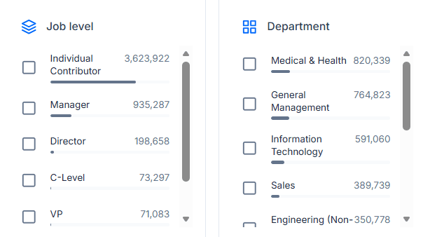
Faceted search powering real-world insights: an example from our customer, DemandScience.
Behind the scenes, each facet corresponds to a column or field in your dataset. Modern search engines use columnar stores to computes how many matching documents belong to each unique value or bucket of that field, then returns both the top results and these aggregate counts in a single response. Because a search result usually returns results that are spread across our dataset the database needs a quick way to look up values for each document.
That duality, returning ranked search hits and category counts, is what makes faceting so powerful. It's also what makes it tricky to implement efficiently in a database built for rows, not documents.
The Problem with Traditional Approaches
If you're thinking, "I'll just run a few extra COUNT queries, how hard can it be?", you're about to discover why search engines exist in the first place.
The thing is, faceting looks simple: it's just grouping and counting. But try to make it fast in a traditional row-based database, and you'll run into serious performance challenges. Want to show search results and category counts from a single query? That's either two index scans or a full index scan and a lot of data transferred. Want it to be responsive? That becomes increasingly difficult as the number of results increases.
Let's take a look at how much faster our approach is, and also how we make this possible (by pipelining the search query and faceting into a single index scan, and making use of a columnar format for value lookups).
Performance: Our Benchmarking Results
As of v0.22.0, the performance of MVCC-accurate faceting is roughly 40% faster.
To demonstrate the performance benefit of our new faceting, we benchmarked traditional PostgreSQL faceting against ParadeDB's integrated approach using a dataset of 46 million Hacker News posts and comments (details on the queries and schema can be found later in the post).
Both approaches use ParadeDB's BM25 search (PostgreSQL's built-in tsvector simply doesn't cut it, already being 27x slower at 200,000 results), but they differ in how faceting is implemented. The results show just how significant the performance difference can be:
ParadeDB Faceting vs Manual Faceting Query Time in Milliseconds
%2C%20ParadeDB%20faceting%20(violet)%2C%20and%20Manual%20faceting%20(blue)%20across%20different%20query%20result%20sizes.%20ParadeDB%20maintains%20consistent%20performance%20while%20manual%20faceting%20degrades%20dramatically%20with%20larger%20result%20sets%2C%20showing%20over%20an%20order%20of%20magnitude%20improvement%20at%20scale%3C/text%3E%3C/svg%3E)
As the chart shows, manual faceting performance degrades dramatically with larger result sets, while ParadeDB's Top K faceting maintains consistent performance by executing both search ranking and aggregation in a single pass through the index. This efficiency comes from making use of ParadeDB's columnar index, which allows fast per-document value lookups during aggregation. At scale, this represents well over an order of magnitude improvement. The orange bar shows ParadeDB with MVCC1 disabled, demonstrating that an additional 3× performance gain is possible when strict transactional consistency isn't required for the facets.
So how does ParadeDB achieve these results? Before we jump into planning and execution let's take a look at our syntax.
Faceting in a Row-Based World
When we set out to design the syntax for faceting, we had three goals:
- Make it intuitive for both SQL users and Elasticsearch users.
- Return both the search results and the facet counts in the same payload as fast as possible
- Integrate cleanly into PostgreSQL's planner and executor.
We experimented with a few approaches: full JSONB result sets, LATERAL subqueries, and a behind-the-scenes UNION. The one we kept coming back to was using PostgreSQL's window functions to express faceting instructions, passing a JSON DSL that mirrors the Elasticsearch aggregation API.
That led us to a new window function, pdb.agg() (also usable in aggregate position, blog coming soon), which accepts JSONB that enables a range of aggregations. Most notably for faceting it supports terms (counting unique values), histograms (bucketing unique values), and date_histogram (bucketing timestamps).
Instead of complex CTEs and multiple queries, you get both search results and facet counts in a single, clean query:
SELECT
  id, title, score, pdb.score(id) AS rank,
  pdb.agg('{"histogram": {"field": "score", "interval": 50}}')
    OVER () as facets
FROM hn_items
WHERE (text ||| 'postgresql')
ORDER BY rank DESC
LIMIT 5;
The magic is the OVER () syntax: this means "over the entire result set, ignoring the LIMIT". This window syntax computes both the top K ranked results and the facet counts in a single pass through the data—exactly the pattern most search applications need.
The result includes both your search hits alongside the faceting data in a JSONB column (effectively overloading this column to contain all the facets). This approach gives you structured, self-contained aggregation results that are easy to parse on the client side.
MVCC and Performance Tradeoffs
By default, ParadeDB maintains full ACID guarantees by checking transaction visibility for every aggregated document. However, for large result sets where approximate counts are acceptable, you can disable MVCC checking for significant performance gains:
-- Default: MVCC enabled (ACID compliant, slower)
pdb.agg('{"terms": {"field": "category"}}') OVER ()

-- MVCC disabled: ~3x faster for large result sets
pdb.agg('{"terms": {"field": "category"}}', false) OVER ()
When MVCC is disabled, the aggregation operates directly on the search index without visibility checks. This is useful for analytics workloads on large datasets where some lag in reflecting the latest updates (bounded by the number of dead tuples since the last VACUUM) is acceptable. But this optional optimization can be great when you need maximum performance or have immutable INSERT only data.
A Complete Example
Let's walk through how this works with a concrete example using our HackerNews dataset:
-- HackerNews table structure
CREATE TABLE hn_items (
    id INTEGER PRIMARY KEY,
    parent_id INTEGER,
    by TEXT,
    text TEXT,
    title TEXT,
    url TEXT,
    type TEXT,
    time TIMESTAMPTZ,
    score INTEGER
    -- ... other columns
);
After creating a ParadeDB search index2, you can run faceted search queries that return both ranked results and category counts:
SELECT
  id, title, score,
  pdb.agg('{"terms": {"field": "type"}}') OVER () as facets
FROM hn_items
WHERE (text @@@ 'paradedb')
ORDER BY score DESC
LIMIT 10;
When you see OVER () alongside an ORDER and LIMIT, it signals: "compute this aggregation over the entire search result set, not just the top K rows returned." This Top K pattern—showing ranked results with facet counts—is exactly what most search interfaces need.
This design intentionally bridges two paradigms. It is designed to be familiar to both Elasticsearch (making use of the Elasticsearch DSL) and SQL (with the WINDOW syntax) users. PostgreSQL's parser treats it as a standard window function call, allowing us to implement custom aggregation logic within the familiar SQL framework.
This design intentionally bridges two paradigms, with the structure of SQL and the flexibility of search engines. It combines the expressiveness of Elasticsearch’s JSON DSL, which allows rich and composable aggregations, with the familiar simplicity of SQL’s WINDOW syntax, which makes it easy to use and reason about. PostgreSQL’s parser treats pdb.agg() as a standard window function call, letting ParadeDB implement custom aggregation logic directly within PostgreSQL’s query execution framework. The result is an interface that feels natural to both SQL and Elasticsearch users.
The first row of the output looks like this:
id     | 41178808
title  | The future of F/OSS continues to be AGPL
score  | 34
facets | {
       |     "buckets": [
       |         { "key": "comment", "doc_count": 185 },
       |         { "key": "story",   "doc_count": 2   }
       |     ],
       | }
The faceting information is added alongside the search query using a JSONB column. JSON is the perfect wrapper for the faceting information: it's structured, self-contained, and easy to parse on the client. Today we attach this to all rows, but in the future, we may optimize this further by returning the facet JSON only on the first row instead of duplicating it.
Comparing the Approaches
Let's see how this compares to a more traditional PostgreSQL approach with the same output, but using complex queries with CTEs and manual aggregations. Both approaches below use ParadeDB for BM25 search, differing in how the faceting is handled. Here's what a very optimized version of "manual faceting" for a histogram of post ratings looks like:
WITH
-- get the id, score and bm25 rank for the search query
hits AS  (
  SELECT
    id,
    pdb.score(id) AS rank,
    score
  FROM hn_items
  WHERE (text ||| 'postgresql')
),
-- do our faceting on the full result-set and build up a JSON object
facets AS (
  SELECT jsonb_build_object(
           'buckets',
           jsonb_agg(
             jsonb_build_object('key', score_bucket, 'doc_count', cnt)
             ORDER BY score_bucket
           )
         ) AS facets
  FROM (
    SELECT
      (score / 50) * 50 AS score_bucket,
      COUNT(*) AS cnt
    FROM hits
    GROUP BY score_bucket
  ) t
),
-- order the original hits by rank and return the top results
limited AS (
  SELECT id, rank FROM hits ORDER BY rank DESC LIMIT 10
)
-- join everything together
SELECT h.id, title, score ,facets
FROM limited h
JOIN hn_items i on i.id = h.id
CROSS JOIN facets f;
Here's what ParadeDB faceting looks like for the same result:
SELECT
  id, title, score, pdb.score(id) AS rank,
  pdb.agg('{"histogram": {"field": "score", "interval": 50}}')
    OVER () as facets
FROM hn_items
WHERE (text ||| 'postgresql')
ORDER BY rank DESC
LIMIT 5;
Same result, simpler syntax, and as we've already seen dramatically better performance.
How Faceting Hooks Into the PostgreSQL Planner
Now we have our syntax, but it isn’t as simple as just writing the pdb.agg() function and calling it a day. Because PostgreSQL aggregates (including those in window functions) usually run after the data is fetched from indexes and loaded to shared buffers we have a problem. We want to do our search and our faceting in a single pass, but they are executed in fundamentally different places during query execution.
PostgreSQL provides a custom scan API that allows extensions to implement their own execution nodes. However, to fully integrate faceting with window functions, we also need to use planner hooks to intercept the planning process before PostgreSQL creates standard window aggregation nodes.
We inject a custom execution node at plan time, intercepting the planning process when we detect a pdb.agg() function used as a window. We do this using a combination of planner hooks and the custom scan API in three stages:
- Query Interception. The planner hook scans the query tree for
WindowFuncnodes usingpdb.agg(). It replaces them with ParadeDB placeholders before PostgreSQL’sgrouping_planner()runs. This prevents Postgres from creating realWindowAggnodes we’d later need to undo. - Custom Scan Injection. When queries combine full-text search,
ORDER BY,LIMIT, and our placeholderWindowAggnode we take over planning. This is the entry point for Top K faceting queries. The planner swaps in aPdbScannode capable of executing both the search and the aggregation in one pass, making sure that the parts of the query that aren’t handled by ParadeDB (non-search WHERE clauses, outer clauses / CTEs, FILTERS) are delegated back to PostgreSQL as normal. - WindowAgg Extraction. Extracts and converts the
pdb.agg()placeholder into a form Tantivy (our underlying search library) understands, adding the information to the customPdbScan. This is where we parse the JSONB definition and build the aggregation tree (terms, range, etc.) to run inside the search engine.
The key insight is timing, this integration happens before PostgreSQL attempts standard window function execution. By execution time the window function doesn’t exist and PostgreSQL is running what it sees as a normal custom scan node.
How Faceting Executes Inside ParadeDB
Once PostgreSQL hands off the plan, the real work begins inside ParadeDB's search layer. At this point, we're no longer working with rows, we're working with search indexes and column data inside Tantivy. The key idea is that ParadeDB executes both ranking and aggregation in the same pass through the index.
1. Searching and Collecting
Every faceting query starts by traversing the search index using the search criteria from the query. We walk through the index entries for matching terms, answering the search part of the query and producing a stream of matching document IDs. This stream forms an ordered iterator representing the candidate documents.
This candidate document stream is then passed into a compound collector, which coordinates all work done over the same stream of documents. This collector runs multiple sub-collectors in parallel, so we can compute different kinds of results (like ranked hits and aggregations) without ever rereading the index.
2. TopDocs Collector (ORDER and LIMIT)
The TopDocs collector is responsible for ranking and limiting the result set. The ranking could be by BM25 score (pdb.score(id), or it could be by a column value (which gets looked up from the columnar storage).
Tantivy uses a quickselect buffer to maintain only the top K highest ordered documents, traversing the document stream and only keeping K records at any one time using a very small amount of memory.
3. Aggregation Collector (Building Facets)
The Aggregation collector is where the actual faceting magic happens. While TopDocs is busy ordering documents, this collector is busy counting things.
For every matching document, the facet collector fetches and aggregates only the fields you asked for (category, price, rating etc.) directly from Tantivy's columnar storage. This matters because we never need to reconstruct full rows like PostgreSQL would, we can pull just the specific column values needed for aggregation, reducing the amount of data we need to read into memory.
Tantivy's columnar storage is designed for exactly this pattern: fast per-document, single-column lookups. For string fields, it uses dictionary encoding, so the entire aggregation happens on integers rather than strings, which are only converted back to strings at the very end. This makes the aggregation process extremely efficient, we're counting integer IDs rather than comparing string values millions of times per second.
Here's where things get interesting from a correctness perspective: this same collector also checks and applies MVCC filtering to maintain full ACID guarantees, only aggregating values that are visible to your current transaction. When the MVCC flag is set to false, we skip these visibility checks entirely for maximum performance, which is useful for analytics workloads where approximate counts are acceptable.
5. Materializing the Final Result
Once collection finishes, ParadeDB has two outputs:
- The ranked hits from the TopDocs collector.
- The facet aggregation result from the Aggregation collector.
The Aggregation collector serializes its in-memory facet map into JSON and attaches it as a single facets column next to the search the query output. This will be mapped back to the value for the pdb.agg() OVER () window.
Conclusion
Faceting is one of those features that looks simple on the surface, but is surprisingly hard to make both easy for developers to use and efficient under the hood. ParadeDB's approach solves this, bringing Elasticsearch-style faceting directly into PostgreSQL. By integrating faceting at the search engine level, we can execute both ranking and aggregation in a single pass through the index, delivering order-of-magnitude performance improvements without forcing you to manage separate search infrastructure.
The result is a simple SQL interface that gives you the best of both worlds: PostgreSQL's ACID guarantees and transactional semantics, combined with the performance and developer experience of modern search engines.
Ready to try faceted search in your PostgreSQL database? Get started with ParadeDB to see how faceting can transform your search experience, and please don’t hesitate to give us a star.
Footnotes
-
MVCC (Multi-Version Concurrency Control) is PostgreSQL's mechanism for handling concurrent transactions by maintaining multiple versions of data when rows are modified. The built in VACUUM asynchronously cleans up these old versions. Accessing rows includes visibility checks in both tables and indexes to ensure each transaction sees the correct version of data. ↩
-
To create a ParadeDB search index, you would run:
CREATE INDEX ON hn_items USING BM25 (id, by, text, title, (url::pdb.literal), (type::pdb.literal), time, score) WITH (key_field=id);. All non-text andliteraltokenized text fields are available to use in faceting. Full documentation on index creation can be found under our CREATE INDEX documentation. ↩